I’ve had a couple of emails recently about the excellent Stanford Machine Learning and AI online classes, so I thought I’d put up the odd post or two on some of the techniques they cover, and what they might look like in PHP.
The second lecture of the ML class jumps into a simple, but often powerful, technique: linear regression - or fitting a line to data (don’t worry if you haven’t watched it, this post hopefully makes sense on it’s own). There are a lot of problems that fall under predicting these types of continuous values based on limited inputs - for example: given the air pressure, how much rain will there be, given the qualifying times, how quick will the fastest lap be in the race. By taking a bunch of existing data and fitting a line, we will be able to make a prediction easily - and often reasonably correctly.
We can define a line with 2 variables, or parameters: the intercept (where it crosses the axis) and the gradient (how much is moves in one dimension for a move of one in the other dimension). Because we’re going to want to predict variables with that line, we’ll write a function that defines it, which, in keeping with tradition, we’ll refer to as our hypothesis function:
<?php
// Return a line function
function hypothesis($intercept, $gradient) {
    return function($x) use ($intercept, $gradient) {
        return $intercept + ($x * $gradient);
    };
}
?>
But which line is the best fit? Intuitively, it is the one closest to the data points we have - which we can measure by taking the square of the different between each predicted value and actual value - we square because then we get positive numbers no matter which way the difference goes:
<?php
// Return the sum of squared errors
function score($data, $hypothesis) {
        $score = 0;
        foreach($data as $row) {
                $score += pow($hypothesis($row[0]) - $row[1], 2);
        }
        return $score;
}
?>
So, our job is to find the line which minimises the squared error - this type of function is referred to the cost function. Lets take our functions above and take a first stab at fitting our line. We’ll write a very simple algorithm which just tests moving each parameter up and down a little bit at a time, and sees if the score gets lower or higher. If it gets lower, we’ll take those parameters and restart the process, until we don’t see any improvement:
<?php
// data x, y
$data = array(
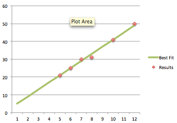
    array(5, 21),
    array(6, 25),
    array(7, 30),
    array(8, 31),
    array(10, 41),
    array(12, 50)
);

function step($data, $params, $min) {
        $minParams = null;

        // Lets calculate our possibilities
        $matrix = array(
                array(0.25, 0),
                array(-0.25, 0),
                array(0, 0.25),
                array(0, -0.25),
        );

        foreach($matrix as $row) {
                $hypothesis = hypothesis($params[0] + $row[0], $params[1] + $row[1]);
                $score = score($data, $hypothesis);
                if( $min == null || $score < $min) {
                        $minParams = array($params[0] + $row[0], $params[1] + $row[1]);
                        $min = $score;
                        echo "New Min: ", $min, "\n";
                }
        }

        return array($minParams, $min);
}

// Starting conditions
$parameters = array(2, 2);
$min = null;
do{
        list($minParams, $min) = step($data, $parameters, $min);
} while( $minParams != null && $parameters = $minParams);

var_dump($parameters);
?>
So for this data, we get the line y = 1 + 4x. If we plot our data and our line on a graph, we can see it’s a pretty good fit:

This algorithm, while straightforward, has several problems. We’re moving in steps of 0.25, so the best answer could be not in this range, and we don’t cache any of our checks, so we’ll always end up evaluating our previous position as a possible move, which is a waste of time. It’s also kind of slow - surely we can do something a bit better?
Of course, we can, and what we can do is use the gradient descent algorithm. This relies on the fact that we are effectively describing a curve with our cost function (or more accurately a curved surface) and we can see how sloped the surface is at any point by taking the derivative, and use the direction of the slope to guide our improvement. In order to use that, we need a bit of calculus to take the partial derivatives for the two parameters, which makes our score function look like this:
<?php
function deriv($data, $hypothesis) {
        $i_res = 0;
        $g_res = 0;
        foreach($data as $row) {
                $i_res += $hypothesis($row[0]) - $row[1];
                $g_res += ($hypothesis($row[0]) - $row[1]) * $row[0];
        }

        $out_i = 1/count($data) * $i_res;
        $out_g = 1/count($data) * $g_res;

        return array($out_i, $out_g);
}
?>
With this new function, we’re going to get a positive or negative value for each field based on the direction, so we know we need to move our values the other way. We can use this in a new step function, which we’ll call gradient. We’re going update our parameters by subtracting the derivative each time, which we’ll multiply by a small learning rate (sometimes referred to as alpha), in order to avoid over-shooting our optimal line.
<?php
function gradient($data, $parameters) {
        $learn_rate = 0.01;
        $hypothesis = hypothesis($parameters[0], $parameters[1]);
        $deriv = deriv($data, $hypothesis);
        $score = score($data, $hypothesis);

        $parameters[0] = $parameters[0] - ($learn_rate * $deriv[0]);
        $parameters[1] = $parameters[1] - ($learn_rate * $deriv[1]);

        // Create a new hypothesis to test our score
        $hypothesis = hypothesis($parameters[0], $parameters[1]);
        if($score < score($data, $hypothesis)) {
                return false;
        }

        return $parameters;
}

do {
        $last_parameters = $parameters;
        $parameters = gradient($data, $parameters);
} while($parameters != false);
var_dump($last_parameters);
?>
What’s cool about this is that we actually get a better result y = 0.29 + 4.08x - which provides a marginally improved score over the 1 and 4 our stepper returned. To be fair, there are easier ways of determining this value mathematically, and things get more interesting if we have more than 2 variables - but we’ll leave that for another post. If you want to see the code for this post in one file, it’s on Github.
