When it comes to classification, and machine learning in general, at the head of the pack there’s often a Support Vector Machine based method. In this post we’ll look at what SVMs do and how they work, and as usual there’s a some example code. However, even a simple PHP only SVM implementation is a little bit long, so this time the complete source is available separately in a zip file.
The classification problem is something we’ve discussed before, but in general is about learning what separates two sets of examples, and based on that then correctly putting unseen examples into one of the other set. An example could be a spam filter, where, given a training set of spam and non-spam mails it is expected to classify email as either spam or not spam.
SVMs are systems for doing exactly that, but they only care about points in spaces, rather than emails or documents. To this end a vector space style model is used to give each word in a document an ID (the dimension) and a weight based on it’s importance to the document (the document’s position in that dimension). Given a series of examples of documents in a vector space, each tagged with a ‘class’ or ‘not class’ designation, the support vector machine tries to find the line that best divides these two classes, and then classifies unseen documents based on which side of the line they appear.
Linearly Separable Classification
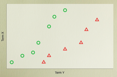
It’s easy to visually separate the two classes above because the problem is in two dimensions. Once we extend this to thousands of dimensions it becomes trickier for a human, but there are a whole bunch of algorithms that will cleanly separate the training cases by defining a line which divides the two sets - but what are makes one solution better than another?
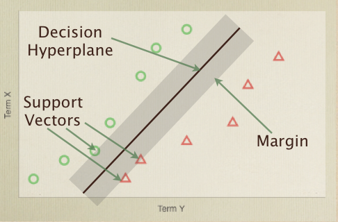
The intuition that drives SVMs is that the line which best divides the two cases is the one that has the largest margin between it and the nearest training examples on either side. Therefore, the important example vectors are the ones that define that margin - the ones closest to the dividing line. These are the support vectors, and it is a combination of them that provides the decision (class or not class) function for an SVM classifier. The function in our example code looks like this:
<?php
protected function classify($rowID) {
        $score = 0;
        foreach($this->lagrangeMults as $key => $value) {
                if($value > 0) {
                        $score += $value * $this->targets[$key] * $this->kernel($rowID, $key);
                }
        }
        return $score - $this->bias;
}
?>
The judgement would then be made whether the score was positive, or negative, which represents which side of the line the document in question was on.
Each of the training examples which supports the dividing line (or more accurately the dividing hyperplane) has a value in the array lagrangeMults which effectively defines it’s weight. The targets array contains which class (represented by +1 or -1) the example was in. The kernel function for now can be thought of as just the dot product between the two vectors.
The final line of the classifier adjusts for a bias value. In a 2D case, a line can be defined as y=ax+b - the b giving you the y intercept at x=0. In the same way a hyperplane has a b (using wTx + b, where w is a vector normal, or perpendicular, to the hyperplane) that specified an offset (so that it does not have to go through the origin), represented by bias. The T stands for Transpose, and is basically taking the dot products between the two vectors.
Effectively we’re trying to learn the weights of the different examples, discarding all the 0 weighted ones (which therefore aren’t support vectors), and calculating the bias. Though not amazingly hard in practice, but does require a bit of maths.
If we take our vector w, which is normal to the hyper plane, then we can say that any the closest point to the hyperplane is _x - yr(w/|w|)_. So that’s saying that the point is vector x minus y (which just changes the sign) times some multiplier r, times the unit version of vector w. The unit version of w is just w divided by it’s length, the length denoted by pipe characters around the vector.
We know that this value must lie on the decision hyperplane, so we can substitute it into the hyperplane equation, then shuffle it around to solve for r:
_r = y * (w<sup>T</sup>x + b / |w|)_
With this then, we can calculate the distance to the boundary for any given example vector, and calculate the margin on our classifier. If we use normalised (length 1) vectors, we can then drop the division and stick with r = y * (wTx + b). We want to make sure there is a margin, so we can define a constraint that r >= 1. We then have an optimisation problem where we have an objective function - that the margin is maximised, and a constraint, r >= 1.
The way this problem is solved is by breaking down the problem. Firstly, maths optimisation problems are always minimisations rather than maximisations, and we can flip this one around by saying we wish to minimise 1/2 wTw. We then specify the constraints as a series of multipliers in the equation, which gives us an equation that the w = ∑ alphaiyixi. ∑ means foreach i in this case, and alpha is the weight, more properly referred to as the Lagrange multiplier. For the bias b = yk-wTxk for any vector x where alphak is not 0.
Of course this does assume that there is a clean dividing hyperplane. This is not always so, as real world data has outliers and misclassified examples, so some tolerance has to be introduced. This is handled by an upper bound on the on the Lagrange multipliers. This allows the optimisation to trade of some misclassification in exchange for a fatter margin.
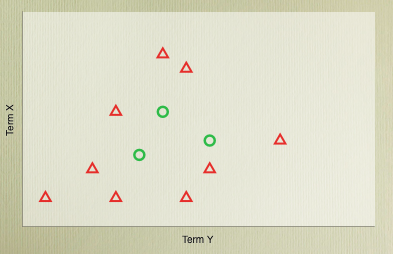
The Kernel Trick
So, with the algorithm we can get the best dividing hyperplane possible, but it’s still, basically, a straight line. This is a problem because there are many problems where a linear classifier simply cannot get good accuracy because of the distribution of the classes in the vector space - there’s simply no straight line or flat plane that can cleanly divide them.
However, the dot product in the SVM classification function doesn’t have to be a dot product. In fact, it can be any function that obeys certain mathematical conditions (function that do are referred to as Mercer kernels), which allows us to plug in another type of function. This kernel function can effectively define a mapping between the dimensions of the problem space, and some higher dimensional space where perhaps the data will be linearly separable.
The function used in our PHP SVM looks like this:
<?php
protected function kernel($indexA, $indexB) {
        $score = 2 * $this->dot($indexA, $indexB);
        $xsquares = $this->dot($indexA, $indexA) +
                        $this->dot($indexB, $indexB);
        return exp(-self::GAMMA * ($xsquares - $score));
}
?>
This is an implementation of a Gaussian Radial Bias Function, which maps onto a space with infinite dimensions. This trick allows good classification results on a variety of different sources, though does come at a cost in terms of extra complexity and computing cost.
Sequential Minimal Optimisation
One of the problems with SVMs is that solving the equation to get the Langragian multipliers for each of the support vectors is a knotty Quadratic Programming problem, and generally requires the used of a specialised library.
People improved the situation by chunking the QP into smaller, more manageable problems, but John Platt took the idea further by breaking the QP down into a series of the smallest possible problems - solving for just a single pair of multipliers at a time. While it will look at more pairs than a more specialised library would have to, each pair can be solved in a fairly straightforward manner. This results in a faster running algorithm in many cases, and because large matrix operations aren’t used the memory usage is much more linear with the number of training examples.
SMO is somewhat complex, but broadly can be broken into three parts. The first is a heuristic for choosing which pair of training examples to optimise, a method for doing the optimisation, and a method for calculating the bias, or b.
The heuristic used to choose the two points starts by examine a given point, then comparing it with the current support vectors. The difference in the results of the two is compared, and point with the highest difference is chosen to optimise against (if there is one).
<?php
foreach($this->lagrangeMults as $id => $value) {
        if($value > 0 && $value < self::UPPER_BOUND) {
                $result2 = $this->errorCache[$id];
                $temp = abs($result - $result2);
                if($temp > $maxTemp) {
                        $maxTemp = $temp;
                        $otherRowID = $id;
                }
        }
}
?>
If this doesn’t find anything then the algorithm chooses any valid support vector that will optimise and uses that. If nothing comes from that loop, it finally just iterates through all the examples looking for one that will optimise. In both cases the start point is randomised.
<?php
$endPoint = array_rand($this->lagrangeMults);
for($k = $endPoint; $k < $this->recordCount + $endPoint; $k++) {
        $otherRowID = $k % $this->recordCount;

        if($this->lagrangeMults[$otherRowID] > 0
                && $this->lagrangeMults[$otherRowID] < self::UPPER_BOUND) {
                if($this->takeStep($rowID, $otherRowID) == 1) {
                        return 1;
                }
        }
}

$endPoint = array_rand($this->lagrangeMults);
for($k = $endPoint; $k < $this->recordCount + $endPoint; $k++) {
        $otherRowID = $k % $this->recordCount;

        if($this->takeStep($rowID, $otherRowID) == 1) {
                return 1;
        }
}
?>
The actual optimisation is performed in the take step function. Initially the classification score is calculated for each point, and an overall score determined by multiplying them together. From that the constraint on the Lagrange multipliers alpha1 and alpha2 is calculated.
<?php
$low = $high = 0;
if($target1 == $target2) {
        $gamma = $alpha1 + $alpha2;
        if($gamma > self::UPPER_BOUND) {
                $low = $gamma - self::UPPER_BOUND;
                $high = self::UPPER_BOUND;
        } else {
                $low = 0;
                $high = $gamma;
        }
} else {
        $gamma = $alpha1 - $alpha2;
        if($gamma > 0) {
                $low = 0;
                $high = self::UPPER_BOUND - $gamma;
        } else {
                $low = -$gamma;
                $high = self::UPPER_BOUND;
        }
}
?>
This is a few lines but is really ensuring that the low value is max(0, $gamma), and the high min(upper bound, $gamma), with the upper bound added to the high example if the classes on the two examples are different, and subtracted from the lower if they’re the same.
Once we have the constraints we need to find the maximum margin while only allowing the two multipliers in question to change. Most of the time we can find the maximum in a straightforward way by dividing the result difference by a value obtained from the maximisation function earlier ($eta in the example).
<?php
$a2 = $alpha2 + $target2 * ($result2 - $result1) / $eta;
if($a2 < $low) {
        $a2 = $low;
} else if($a2 > $high) {
        $a2 = $high;
}
?>
Calculating the other multiplier is pretty straightforward, most of the time, from looking at the original multipliers and the new $a2 multiplier.
<?php
$a1 = $alpha1 - $score * ($a2 - $alpha2);
?>
The bias (b) update is pretty simple once the new Lagrange multipliers have been determined. A bias is calculated for each based on the current bias, and the change in multiplier. If both are valid then the average of the two new biases is used, else only the bias generated from the valid multiplier is.
<?php
$b1 = $this->bias + $result1 +
        $target1 * ($a1 - $alpha1) * $k11 +
        $target2 * ($a2 - $alpha2) * $k12;
$b2 = $this->bias + $result2 +
        $target1 * ($a1 - $alpha1) * $k12 +
        $target2 * ($a2 - $alpha2) * $k22;
if($a1 > 0 && $a1 < self::UPPER_BOUND) {
        $newBias = $b1;
} else if($a2 > 0 && $a2 < self::UPPER_BOUND) {
        $newBias = $b2;
} else {
        $newBias = ($b1 + $b2) / 2;
}
$deltaBias = $newBias - $this->bias;
$this->bias = $newBias;
?>
Using The Classifier
The classifier is pretty straightforward to use, as longs the data is formatted appropriately. The format for the data is based on the svmlight format, and is pretty convenient for text classification - all that is needed is an ID for each term, and a unit length document vector. The format is:
+1 1:0.049 45:0.029…..
With the first entry being +1 or -1 for the two classes (or 0 for data to be classified), and then pairs of key:value entries in increasing dimension order. The data doesn’t have to be continuous though - dimensions with value 0 can be omitted.
Using the example data in the zip file, we can trigger it to train:
<?php
$svm = new PHPSVM();
$svm->train('data/train.dat', 'model.svm');
?>
And to classify, which you’re likely to do repeatedly (though for testing train function can actually take the data path as a third argument):
<?php
$svm = new PHPSVM();
$svm->test('data/test.dat', 'model.svm', 'output.dat');
?>
This will output the results for each input to the output.dat file, and print an overall accuracy if the test data has judgements along with it. It gives a pretty good result, though it’s worth noting that the included training and test data are well balanced (similar numbers of positive and negative examples), so your mileage may vary.
Accuracy: 0.92976588628763 over 598 examples.
For more complex usage, or for more examples where memory limits becomes an issue, you will probably want to use one of the excellent SVM systems available such as LibSVM / LibSVM+ or SVMlight (though SVMlight is only free for non-commercial user). These offer great speed and accuracy, and are at the cutting edge of extensions to the algorithms. However, it may be preferential to actually classify examples in PHP using a model generated by one of those systems, which is quite doable.
Special thanks to Lorenzo and Vincenzo for their comments about the PHPSVM class.