Classification techniques are used for spam filters, author identification, intrusion detection and a host of other applications. They can be used to help organise data into a structure, or to add tags to allow users to find documents. While the latest classification algorithms are at the cutting edge of machine learning, there are still thousands of systems using simpler algorithms to great effect.
Classification is the process of assigning items, usually documents of one form or another, to groups from a predefined set. Unlike clustering the groups are (usually) known before hand, and rather than attempting to work out the groupings by looking at the data the classifier is trained by examining examples of documents in each group - referred to as supervised learning, as opposed to clustering’s unsupervised learning.
Because it’s more interesting to work with real data, even if the problem is a toy one, we’ll look at two classification algorithms and how they can solve the vitally important Twitter author identification problem - specifically whether they can tell the different between the tweets of Cal Evans and Ivo Jansch. Both update fairly frequently, and have some similar interests, but are pretty easy for a human to tell apart - Cal rarely speaks dutch for example! The question is whether an algorithm can do the same, and if so, how reliably.
Data
The first thing we’ll need is to collect and divide the data. We can grab the data from twitter pretty easily, but for the purposes for the experiment we’ll exclude retweets (reposting another user’s twitter message), which is pretty easy to do thanks to the convention of putting RT at the start of such posts. I took 100 tweets each from Cal and Ivo, which you can find in this zip file.
Next we have to divide the collected data into two sets - one for training the classifier, and one for testing it. This tests the classifier’s ability to generalise - if we trained and tested on the same data we might find that while we get good results on that, our results on new, never seen, data aren’t half as good.
Rocchio
The first, simple, algorithm we’ll look at is the Rocchio classifier. The theory behind the classifier is pretty simple: if we average together the tf-idf vectors of all the documents in each group, we’ll end up with one centroid per group. We then compare the document in question to our averaged group centroids, and assign the document to the group it is most similar too.
Twitter isn’t a particularly easy data set to work with though. Tweets are short - limited to 140 characters - so the term frequency of a given term is usually 1. This means all the onus goes on the inverse document frequency, which still works, but the overall weighting loses some power due to the lack of a local component.
A twitter specific weighting scheme might perform better, by increasing the weight for #tags for example, as they are usually contextually significant. Some decent preprocessing may be rewarded by good performance as well, stripping out URLs for example. For this case though, we’ll just take the data straight, and see how we do.
Below is a quick and dirty Rocchio class:
<?php
class Rocchio {
        protected $dictionary = array();
        protected $documents = array();
        protected $classes = array();
        protected $docToClass = array();
        protected $docCount = 0;
        protected $centroids = array();
        protected $results = array();

        public function addDocument($document, $class) {
                preg_match_all('/\w+/', $document, $matches);
                $docID = ++$this->docCount;
                $this->classes[$class][] = $docID;
                $this->docToClass[$docID] = $class;

                foreach($matches[0] as $match) {
                        $match = strtolower($match);
                        if(!isset($this->dictionary[$match])) {
                                $this->dictionary[$match] =0;
                        }
                        if(!isset($document[$docID][$match])) {
                                $this->dictionary[$match]++;
                                $this->documents[$docID][$match] = 0;
                        }

                        $this->documents[$docID][$match]++;
                }
        }

        public function test($document, $testClass) {
                $document = $this->linearise($document);

                foreach($this->centroids as $class => $terms) {
                        $score[$class] = 0;
                        foreach($terms as $term => $termScore) {
                                if(isset($document[$term])) {
                                        $score[$class] += $termScore *
                                                (log($document[$term], 2) +
                                                (log($this->docCount
                                                        / $this->dictionary[$term], 2)));
                                }
                        }
                }

                arsort($score);
                $result = key($score);

                if($result == $testClass) {
                        $this->results['true'][$result] += 1;
                } else {
                        $this->results['false'][$result] += 1;
                }
        }

        public function train() {
                foreach($this->classes as $class => $documents) {
                        $classCount = count($this->classes[$class]);
                        $total = 0;
                        foreach($documents as $docID) {
                                $terms = $this->documents[$docID];
                                foreach($terms as $term => $count) {
                                        $score =
                                                 (1 / $classCount) *
                                                ( log($count, 2)
                                                + log($this->docCount
                                                        / $this->dictionary[$term], 2));
                                        $this->centroids[$class][$term] += $score;
                                        $total += $score;
                                }
                        }
                        $this->centroids[$class] =
                                $this->normalise($this->centroids[$class], $total);
                }
        }

        public function getStats() {
                // fancy output is for suckers.
                var_dump($this->results);
        }

        protected function linearise($input) {
                preg_match_all('/\w+/', $input, $matches);
                $document = array();
                foreach($matches[0] as $match) {
                        $match = strtolower($match);
                        if(!isset($document[$match])) {
                                $document[$match] = 0;
                        }
                        $document[$match]++;
                }
                return $document;
        }

        protected function normalise($vector, $total) {
                foreach($vector as &$value) {
                        $value = $value/$total;
                }
                return $vector;
        }
}
?>
The key function here is train. This sums the vectors in each group, multiplying the values by 1 over the count of documents in that class to get the center of the group of points. Add document is really just chopping up the documents to prepare for the training, and the test function looks for the most similar match between the centroids at the supplied document. It does this by taking the dot product between the centroid vectors and the document, and looking for the one with the highest score, calculating the cosine of the angle between the two vectors.
We can run this by reading in the files we had earlier:
<?php
$rocchio = new Rocchio();
$cal = file_get_contents('calevans.txt');
$ivo = file_get_contents('ijansch.txt');
$cal = explode("\n", $cal);
$ivo = explode("\n", $ivo);
for($i = 0; $i < count($cal)-1; $i += 2){
        $rocchio->addDocument($cal[$i], 'calevans');
        $rocchio->addDocument($ivo[$i], 'ijansch');
}
$rocchio->train();
for($i = 1; $i < count($cal); $i += 2) {
        $rocchio->test($cal[$i], 'calevans');
        $rocchio->test($ivo[$i], 'ijansch');
}
$rocchio->getStats();
?>
Evaluating The Classifier
The first step in evaluating the classifier is to work out four numbers:
- True positive: where the judgement was positive and correct
- True negative: where the judgement was negative and correct
- False positive: where the judgement was positive, but incorrect
- False negative: where the judgement was negative, but incorrect
In our example, we’d probably replace “positive” and “negative” with Cal and Ivo (or vice versa), but either way we can then calculate some values.
The simplest is the accuracy: the number of right judgments over wrong judgments.
<?php
function accuracy($tp, $fp, $tn, $fn) {
        return ($tp + $tn) /  ($tp + $fp + $tn + $fn);
}
?>
Accuracy is good - but it’s not necessarily enough. For example, with a spam checker we might be much more worried about false positives (where a good email is classified as spam) than a false negative (where a spam is given the all clear). Seeing an extra spam message is irritating, but missing an important email because your checker though it was spam is much worse. This is a tradeoff between precision - the measure of how reliable a positive judgment is, versus recall - the measure of what percentage of available positives are accurately judges as so.
<?php
function precision($tp, $fp, $tn, $fn) {
        return $tp / ($tp + $fp);
}

function recall($tp, $fp, $tn, $fn) {
        return $tp / ($tp + $fn);
}
?>
Generally, preferring one comes at the cost of the other - in the extreme it’s easy to get a high score on one by decimating the other. To get a great precision, just take the documents you’re the most of sure about, but that means plenty of genuine positives will slip by, giving you a bad recall. To get a good recall, simply mark everything as positive - the recall will be perfect, but the precision not so much.
To balance these two, the Fβ measure uses both values, and allows weight towards one or another, through the beta value. If beta is 0.5, recall is half as important as precision, as might be wanted for the spam checker, for example.
<?php
function fbeta($precision, $recall, $beta = 1) {
        return
                (($beta + 1) * $precision * $recall) /
                (($beta * $precision) + $recall);
}
?>
Looking at the stats from our Rocchio classifier we come up with these values:
array(2) {
  ["true"]=>
  array(2) {
    ["calevans"]=>
    int(38)
    ["ijansch"]=>
    int(32)
  }
  ["false"]=>
  array(2) {
    ["calevans"]=>
    int(18)
    ["ijansch"]=>
    int(12)
  }
}
This gives us an accuracy of 38+32 / 38+32+18+12 = 0.7. Precision is 38 / 38 + 18 = 0.67 and Recall 38 / 38 + 12 = 0.76, so our algorithm naturally prefers recall slightly to precision. The f-measure (for beta 1) is 2 * 0.67 * 0.76 / 1 * 0.67 + 0.76 = 0.71 - which is the score we’ll want to consider. A good score here would be in the 0.8-0.9 range, with the state of the art getting in the 0.9 range. Still, there isn’t a great deal of data for training or testing, and I suspect with some more time and tweaking this could get up to the high 0.7s.
Perceptron
The next algorithm is derived from one of the earliest types of neural network, the perceptron. The algorithm works by iteratively improving a guess of which line would best divide the examples, learning by updating the line each time it gets it wrong.
Unfortunately, if there is not a perfect dividing line available, the algorithm will bounce around and not give great results. To solve this, the voted perceptron was invented, which works the same but keeps all the intermediate guesses, and a count of how often they were correct, and tests the document under question against all of them, weighting them against how much they were succesful. Because this can be somewhat slow, the algorithm we’ll be using is the averaged perceptron - this will average all the tested model vectors by their weights into a single vector, much like Rocchio did with the training vectors themselves.
<?php
class AveragedPerceptron extends Rocchio {
        protected $model;

        public function train() {
                $allModels = array();
                // Get our classes
                $classIDs = array_keys($this->classes);
                if(count($classIDs) > 2) {
                        die('This class only handles binary classification');
                }

                // Initialise model to random array.
                $model = array();
                $total = 0;
                foreach($this->dictionary as $term => $df) {
                        $model[$term] = rand(0, 10000) / 10000.00;
                        $total += $model[$term];
                }
                $model = $this->normalise($model, $total);

                // Do the actual training!
                for($loop = 0; $loop < 2; $loop++) {
                        foreach($this->documents as $docID => $terms) {
                                // test whether we classify this correctly
                                $result = intval($this-> calcAndDotProd($terms, $model) > 0);
                                if($classIDs[$result] == $this->docToClass[$docID]) {
                                        // if we get it right, this model is good
                                        $allModels[] = $model;
                                } else {
                                        // if the prediction was wrong, update the model
                                        $sign = $result == 1 ? -1: 1;
                                        foreach($terms as $term => $value) {
                                                $model[$term] += $sign * $value;
                                                $total += $value; // abs
                                        }
                                        $model = $this->normalise($model, $total);
                                        $allModels[] = $model;
                                }
                        }
                }

                $total = 0;
                foreach($allModels as $model) {
                        foreach($model as $term => $val) {
                                $this->model[$term] += $val;
                                $total += $val;
                        }
                }
                $this->model =$this->normalise($this->model, $total);
        }

        public function test($document, $class) {
                $classIDs = array_keys($this->classes);
                $document = $this->linearise($document);
                $result = intval($this-> calcAndDotProd($document, $this->model) > 0);
                if($classIDs[$result] == $class) {
                        $this->results['true'][$class] += 1;
                } else {
                        $this->results['false'][$class] += 1;
                }
        }

        protected function calcAndDotProd($vectora, $vectorb) {
                $score = 0;
                foreach($vectora as $key => $val) {
                        if(isset($vectorb[$key])) {
                                $val = (log($val, 2) +
                                                (log($this->docCount
                                                        / $this->dictionary[$key], 2)));
                                $score += $val * $vectorb[$key];
                        }
                }
                return $score;
        }
}
?>
The train method is again the key part of the algorithm. After initialising the model to a random vector, it steps through each training example testing whether it would classify it correctly. If so, the model is stored, if not the model is updated by adding the example it got wrong, in the appropriate direction. Once all the training examples have been seen, all the stored models are averaged together to give the final model, which is then used to test examples. In this case we actually loop over the training data twice, to give the model a chance to hone in on the preferred line, which helps smooth out the classification.
Because the model is the dividing hyperplane between the two classes of data, when we take the dot product, we aren’t testing for similarity in the same way as with Rocchio. Instead we’re looking for which side of the line the document falls, which we determine by looking at the sign - whether or not the result of the dot product is positive.
!!Evaluating The Averaged Perceptron
array(2) {
  ["true"]=>
  array(2) {
    ["calevans"]=>
    int(39)
    ["ijansch"]=>
    int(38)
  }
  ["false"]=>
  array(2) {
    ["ijansch"]=>
    int(12)
    ["calevans"]=>
    int(11)
  }
}
Here the precision is 39/39+11 = 0.78 and the recall 39/39+12 = 0.76 so the f-measure is an improvement over Rocchio at 2 * 0.78 * 0.76 / 0.78 + 0.76 = 0.77. That said, this algorithm can also do a lot better, if some time was taken and the data improved.
Linear Classifiers
Both of the classifiers we’ve looked at here will work best if the data is linearly separable so that literally a line (or more accurately a hyperplane) can be drawn through the document space that has all of one group on one side, and all of the other group on the other side.
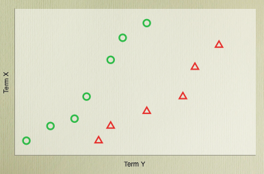
In 2D, this is the kind of case we’re looking for. The Rocchio algorithm attempts to find this line by finding the middle point of the example cases, while the Perceptron more explicitly looks for the dividing line. If such a line is available, the Perceptron should eventually find it, but most real world data isn’t really cleanly separable. The worst kind of cases can really resist linear separation:
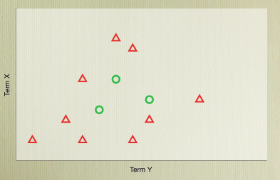
In this case the best move is to look at other classifiers, which are better able to handle diverse data. These range from the relative simple, such as K-Nearest Neighbour, to the really very complicated, such as Support Vector Machines. The perceptron itself can even be extended to handle non-linearly separable cases, but that’s something for another post!